Introduction
Open software distance matrix computation is the use of open-source or openly accessible routing engines and map data to calculate travel distances and/or times between every pair of locations in a set, producing a structured table of pairwise costs without relying on a closed, proprietary provider. The operational consequences of getting it wrong are concrete and costly.
This guide is written for logistics engineers, route optimization developers, and fleet operations teams who need to understand distance matrix computation end-to-end — as a production system with real accuracy and scale requirements.
Bad matrix computation doesn't just produce suboptimal routes — it produces infeasible ones:
- A 13-foot truck routed under a 12-foot bridge
- Stops sequenced by straight-line distance that ignore one-way streets
- Time windows missed because 6am traffic conditions were applied to a 5pm dispatch
What follows covers how the process works, what affects computation quality at scale, and where teams consistently go wrong when integrating distance matrix APIs into routing systems.
Key Takeaways
- A distance matrix is an N×N (or M×N) table of pairwise travel costs — distance, time, or both — between a set of locations.
- VRP, TSP, and CVRP solvers all require a distance matrix before stop sequencing can start.
- Road-network distance is required for logistics accuracy; straight-line (haversine) approximations are insufficient for production routing.
- Scale hits fast: 500 locations means 250,000 pairwise calculations.
- Standard APIs cap at 25×25 entries — a hard ceiling that breaks down for real-world fleet operations.
What Is Distance Matrix Computation?
A distance matrix is an N×N (or M×N) table where each cell contains the travel cost — distance, time, or a combination — between a specific origin-destination pair. Diagonal values are always zero: the cost of traveling from a point to itself.
The purpose of computing this matrix isn't academic. It transforms a flat list of locations into a complete, queryable cost structure that downstream algorithms can consume to make optimal assignment and sequencing decisions. Without it, a VRP solver has no way to evaluate whether visiting Stop A before Stop B saves time or adds it.
Distance Matrix vs. Route: Not the Same Thing
The two are often confused, but they serve different purposes:
- Distance matrix: Computes pairwise costs for all combinations in bulk, with no specified sequence
- Route calculation: Calculates an ordered path for a specific trip between defined waypoints
They are complementary inputs, not interchangeable tools. Compute the distance matrix first; route planning consumes its output. Using turn-by-turn routing APIs to simulate matrix computation (one call per pair) is slower, more expensive, and doesn't return the structured 2D array that solvers require. Teams evaluating open software distance matrix computation should confirm the engine returns this structured array natively, rather than requiring a wrapper script to stitch together individual route calls.
Why Distance Matrix Computation Is Critical in Logistics
VRP, TSP, and CVRP solvers are mathematically dependent on a complete cost matrix before sequencing can begin. The solver's job is to evaluate thousands of possible stop orderings and find the minimum-cost assignment. That evaluation requires knowing the cost of every possible pair transition — which is exactly what the matrix provides.
Real logistics operations make this harder, not easier:
- 50–500+ stops per vehicle per day
- Multiple depots with variable starting points
- Strict time windows for delivery or service
- Vehicle-specific road restrictions (weight limits, height clearances, hazmat regulations)
All of these require accurate pairwise costs pre-computed at scale. A matrix that ignores truck routing restrictions or models traffic at the wrong time of day produces route plans that drivers cannot execute on the road.
The Cost of Getting It Wrong
Research on vehicle routing on road networks shows that Euclidean approximations underestimate actual road travel costs, with the gap widening in dense urban environments and areas with complex road topology.
Routes built on straight-line approximations ignore bridges, toll restrictions, one-way streets, and truck height limits — generating plans that look optimal in the algorithm but are undeliverable on the road.
How Distance Matrix Computation Works
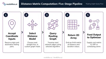
The process follows a consistent sequence across all tools and APIs:
- Accept coordinate inputs — origins (depots, driver locations) and destinations (delivery stops, job sites)
- Select a distance model — straight-line approximation or road-network routing
- Query the routing graph or API — run shortest-path calculations for each origin-destination pair
- Return a structured 2D array — rows = origins, columns = destinations, values = travel cost
- Feed output to the optimizer — the matrix becomes the cost input for the VRP/TSP solver
Step 1: Define Origin and Destination Sets
Origins and destinations are passed as coordinate pairs (latitude, longitude). For asymmetric use cases (say, 20 drivers mapped against 300 delivery stops), the matrix is M×N rather than square. This is standard in fleet dispatch.
Two preprocessing details matter here:
- Duplicate locations inflate matrix size unnecessarily; deduplicate before calling the API
- Snap-to-road corrects coordinates that don't sit on the road network (a GPS point in the middle of a building, for example), which affects whether the routing engine can find a valid path at all
Step 2: Select the Routing Model and Cost Metric
This is where most misconfiguration happens. Key decisions:
| Parameter | Options | Logistics Implication |
|---|---|---|
| Vehicle profile | Car, truck, motorcycle | Truck profiles enforce height/weight/hazmat restrictions |
| Optimization objective | Fastest vs. shortest | Time-based matrices align with delivery windows |
| Traffic model | Real-time, historical, static | Affects time-window accuracy significantly |
| Cost metric returned | Seconds/minutes, meters | Most logistics ops prefer time over raw distance |
Truck-specific routing is non-negotiable for commercial fleets. A car profile ignores weight limits, height restrictions, and hazmat regulations, producing matrices that route heavy vehicles onto roads they legally cannot use.
Step 3: Execute the Query and Consume the Result
The routing engine runs shortest-path calculations across the road graph for each origin-destination pair. Modern engines use algorithms like Contraction Hierarchies, which preprocess the road graph to significantly speed up query times compared to running Dijkstra's algorithm from scratch on every pair.
The API returns a 2D array:
- Rows = origins
- Columns = destinations
- Cell values = travel cost (time in seconds/minutes, distance in meters, or both)
Key Factors That Affect Distance Matrix Computation Performance
Input Scale and Matrix Dimensions
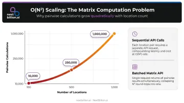
Matrix complexity grows as O(N²). At 100 locations, you have 10,000 pairwise calculations. At 500 locations, that's 250,000. At 1,000, it's 1 million.
This quadratic scaling is why naive sequential API calls — one per origin-destination pair — are not operationally viable at fleet scale. The latency adds up, error handling compounds, and per-call costs multiply quickly. Purpose-built matrix APIs batch this computation in a single request, which is architecturally the only approach that works at production scale.
Road Network Data Quality
Matrix accuracy depends on the freshness of the underlying map data. Outdated road graphs produce incorrect costs — particularly in:
- Emerging markets with rapidly changing infrastructure
- Areas with recent road construction or closures
- Regions where OpenStreetMap coverage is incomplete
OpenStreetMap's road coverage globally exceeds 80%, but coverage quality varies by region. For logistics operations in markets with lower OSM completeness, map data source and update frequency become critical selection criteria for any distance matrix provider. Open software distance matrix computation built on OpenStreetMap gives teams visibility into the underlying map data and the ability to patch or contribute corrections directly, which is not possible with closed commercial datasets.
Vehicle Profile Specificity
A matrix computed for a standard car profile will differ materially from one computed for a heavy truck with height and weight restrictions. The difference isn't just in speed — it's in route validity. Truck-specific routing enforces constraints that consumer profiles ignore entirely, including:
- Bridge weight limits
- Tunnel height clearances
- Hazardous material transport corridors
- Urban delivery zone restrictions
Using the wrong profile produces a matrix where the computed paths are physically infeasible on the road network.
Traffic and Time-of-Day Modeling
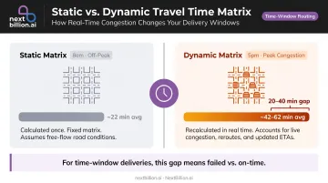
Static matrices assume constant travel conditions — which is never true in practice. Dynamic matrices incorporating real-time or historical traffic patterns produce meaningfully different time estimates, particularly for operations with strict delivery windows.
The gap between a static 8am matrix and actual 5pm conditions can be 20–40 minutes on dense urban routes. For time-window-constrained deliveries, that difference is the difference between on-time and failed.
API Size Limits and Architecture
Most general-purpose mapping APIs cap matrices at 25×25 or 100×100 entries per request. For a fleet with 200 stops, this forces teams to stitch together dozens of partial API calls — introducing latency, error-handling complexity, and per-call cost multiplication.
Google's Distance Matrix API and Mapbox's Matrix API both operate under these constraints. For teams building production routing systems, the ceiling matters more than the average case.
NextBillion.ai's Distance Matrix API supports matrices up to 5,000×5,000 elements in a single call (up to 25 million origin-destination pairs), with 2–3x lower latency and 10–20x higher throughput compared to standard alternatives. For a Canadian fleet management platform serving over 4 million connected vehicles, this eliminated the need for batched calls and achieved 95% accurate arrival times using predictive ETA modeling.
Common Misconceptions and Pitfalls
"Haversine is good enough for our use case"
Haversine calculates the great-circle distance between two coordinates — the shortest path on a sphere. It's fast and useful for geographic clustering. It is not accurate for route planning.
Haversine cannot account for:
- One-way streets
- Road closures or restricted access
- Actual road geometry (a river with one bridge forces a detour haversine ignores)
- Truck-specific route restrictions
For rough geographic grouping before optimization, haversine is fine. As the cost input to a VRP solver, it produces systematically incorrect route plans.
Using Turn-by-Turn APIs to Build a Matrix
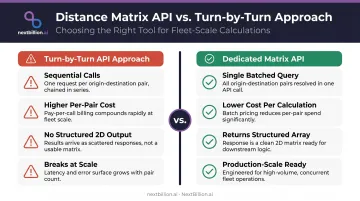
Some teams try to construct a matrix by calling a directions API for each origin-destination pair individually. This approach:
- Takes longer due to sequential API calls
- Costs more per calculation than a dedicated matrix API
- Does not return the structured 2D array that optimization solvers require
- Breaks at any meaningful scale due to latency accumulation
A dedicated matrix API runs all pairs in a single optimized query. The difference is architectural: batched computation versus repeated single-pair lookups that compound in both cost and latency.
Caching a Static Matrix Indefinitely
Even a well-built matrix has a shelf life. A matrix computed at 6am is not accurate at 4pm — traffic conditions, road incidents, and time-of-day routing differences all erode its accuracy the further dispatch moves from computation time.
Teams should either:
- Compute matrices close to the time of dispatch
- Use time-of-day-aware APIs that accept a departure time parameter
- Re-compute dynamically for same-day delivery workflows
Stale matrix data is one of the more common root causes of planned-versus-actual route divergence in same-day operations.
When a Standard Distance Matrix API Falls Short
Generic mapping APIs are built for consumer use cases. The constraints they impose — 25×25 matrix caps, per-call pricing, no truck routing — reflect that design intent. They work for getting driving directions. They don't work for operating a fleet.
Scale Ceiling Problems
When fleet sizes exceed consumer API limits, teams face a choice: stitch together dozens of partial calls (expensive, slow, error-prone) or find an API built for the workload. A US-based trucking logistics startup making millions of matrix calls monthly achieved a 30% reduction in API costs after switching to a purpose-built logistics API — without sacrificing performance or accuracy.
The per-call pricing model compounds the problem. As delivery volumes increase seasonally, per-call costs scale proportionally. At high volume, the cost structure of standard mapping APIs becomes unsustainable at scale.
Scenarios That Require Purpose-Built Infrastructure
Standard APIs are also architecturally unsuited for:
- Real-time dynamic re-optimization — same-day delivery with new order insertions requires low-latency re-computation that standard endpoints aren't designed to support
- Multi-depot planning at scale — hundreds of vehicles across multiple starting points require large asymmetric matrices and truck-compliant routing simultaneously
- On-premise deployment — operations with data privacy requirements (healthcare, government, enterprise logistics) need APIs deployable within their own Kubernetes environment or private data center
NextBillion.ai's Distance Matrix API is built for these workloads:
- Large matrix computation with no 25×25 cap
- Truck-compliant routing profiles
- Real-time and historical traffic modeling
- Sub-second response times
- Cloud-hosted and on-premise deployment options
For a European TMS provider, that combination translated to a 30% improvement in ETA accuracy and 40% savings on API expenses compared to their previous provider.
Conclusion
Distance matrix computation transforms a list of locations into the structured cost table that every route optimizer, job scheduler, and dispatch system depends on. Get it right, and downstream decisions — stop sequencing, driver assignment, time-window compliance — are made on accurate data. Get it wrong, and those errors propagate through every decision in the planning stack.
Four configuration choices determine whether the routes your system produces are physically executable: vehicle profile (car vs. truck), traffic model (static vs. dynamic), matrix dimensions (does your API cap at 25×25?), and update frequency. Treat them as implementation details at your own risk.
Choose your computation approach based on actual operational requirements, not on what's easiest to access. For teams moving beyond consumer-grade APIs into production fleet operations, the differences add up fast: no matrix size caps, truck-specific routing constraints, and traffic models that reflect real road conditions rather than averaged estimates. Tools like NextBillion.ai's Distance Matrix API are built specifically for this layer — so the data feeding your optimizer reflects how vehicles actually move, not how passenger cars do.
Frequently Asked Questions
What is the difference between a distance matrix and a travel time matrix?
A distance matrix returns spatial distance (meters or miles) between location pairs, while a travel time matrix returns duration (seconds or minutes). Most logistics operations prefer time-based matrices because delivery windows and driver schedules are time-constrained, not distance-constrained — a 10-mile route in congested traffic takes longer than a 15-mile highway route. This matters for US fleets managing FMCSA hours-of-service limits, where driver time on duty, not miles driven, is the constraint being planned against.
What is the maximum matrix size supported by distance matrix APIs?
Limits vary significantly by provider. Consumer-grade APIs like Google's Distance Matrix API cap at 25×25 entries per request; Mapbox's Matrix API caps at 10×10. Enterprise logistics APIs are designed for much larger workloads — NextBillion.ai supports up to 5,000×5,000 elements in a single request. Verify size limits before building a production routing system.
How does a distance matrix feed into route optimization and VRP solvers?
VRP and TSP solvers consume the distance or time matrix as their cost input, using it to evaluate all possible stop sequences and find the minimum-cost assignment. Without a complete matrix, the solver cannot compare route alternatives or produce an optimal solution.
What is the difference between Euclidean distance and road network distance in a matrix?
Euclidean (straight-line) distance ignores roads, terrain, one-way streets, and vehicle restrictions. Road network distance follows the actual drivable path on the map graph. For any logistics planning that produces real driver routes, road network distance is required. Euclidean distance is only appropriate for rough geographic clustering before optimization runs.
How long does it take to compute a large distance matrix?
Computation time depends on matrix size and the routing engine. Modern APIs using Contraction Hierarchies process thousands of elements in seconds — NextBillion.ai handles many thousands of elements in roughly 5 seconds, with larger workloads completing in around 100 seconds. Naive sequential API call approaches can take hours for equivalent workloads.
Can a distance matrix be computed in real time for dynamic routing?
Real-time matrix computation is used in same-day delivery and on-demand dispatch scenarios where new orders arrive continuously. It requires a purpose-built logistics API with high-throughput ingestion, real-time traffic data, sub-second response times, and a 99.9% uptime SLA — standard mapping endpoints are not architected for this use case. Dispatch systems recomputing matrices on the fly also need to account for live traffic incidents and road closures, since stale distance data leads to route plans that no longer reflect actual driving conditions on the ground.
What open-source options exist for computing a distance matrix?
Open-source routing engines such as OSRM, Valhalla, and GraphHopper can compute distance and time matrices from OpenStreetMap data. They give teams full control over the routing graph and are free to self-host, but require infrastructure to run, maintain, and scale, plus ongoing work to keep map data, traffic, and road restrictions current. Commercial APIs trade that operational overhead for managed infrastructure and support.