Introduction
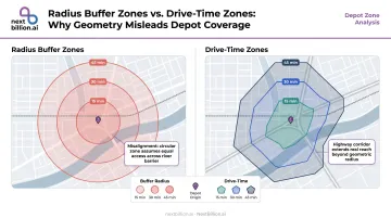
Picture two logistics planners designing delivery zones around the same depot. The first draws a 10-mile radius circle — clean, symmetrical, done in seconds. The second generates a drive-time polygon. Their output looks nothing like a circle: it stretches far along an interstate to the northwest, retracts sharply where a river cuts off road access to the east, and shows realistic reach in every direction based on actual roads.
The first planner will over-serve customers near highway corridors while under-serving others across town who are technically "within range" but 45 minutes away by road. The second planner's zones reflect where drivers can actually go.
That gap between assumed reachability and actual road-network reachability is exactly what drive-time polygons solve. This guide covers the definition, computation mechanics, practical use cases, generation methods, and accuracy factors.
Key Takeaways
- Drive-time polygons enclose all road-accessible locations reachable from a starting point within a set time or distance, shaped by road topology rather than a straight-line radius.
- They're computed using graph traversal (Dijkstra's algorithm) against a weighted road network dataset.
- Core use cases: delivery zone tiering, field service territory design, retail site selection, emergency response coverage.
- Generation options: desktop GIS platforms (ArcGIS Pro, QGIS) for analysis work; API-based services for programmatic, production-scale generation.
- Accuracy depends on road network data quality, traffic model type, and vehicle routing constraints applied.
What Are Drive-Time Polygons?
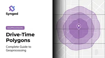
A drive-time polygon encloses all road-accessible locations reachable from a starting point within a set time or distance. Unlike a simple radius circle, its shape is determined by actual road topology, stretching further along highways and retracting where roads are limited or blocked. A drive-time polygon (also called a service area polygon or isochrone, from Greek isokhronos: equal time) is a geographic region enclosing every point reachable from a single origin by vehicle travel within a defined time or distance threshold. The shape is irregular by design: it follows road topology rather than radiating uniformly from a center point. Generating these polygons programmatically at scale is typically done through an API-based service rather than manual desktop GIS work, as covered later in this guide.
Why Radius Buffers Fall Short
A straight-line radius buffer assumes travel at equal speed in all directions regardless of what's actually on the ground. That assumption breaks down fast.
Research published in Health Services Research analyzing 66,492 members found that median drive distance was 11.9 miles while the equivalent Euclidean (straight-line) distance was just 9.5 miles — and the maximum absolute difference between the two measures reached approximately 146 miles in cases where road networks diverge sharply from straight-line paths. Mountains, rivers, rail lines, and highway access points all create this divergence.
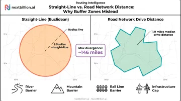
For operations work, that's not a minor rounding error. Zones built on straight-line buffers consistently misallocate workload — overpromising coverage in some areas, undercutting capacity in others.
Rings vs. Disks: Two Output Modes
When generating polygons at multiple break values (say, 10, 20, and 30 minutes), you choose between two output modes:
- Disks — cumulative polygons showing all reachable area up to each threshold. The 30-minute disk contains everything reachable within 10, 20, and 30 minutes.
- Rings — incremental bands showing only the area between consecutive thresholds. The 20–30 minute ring shows only what's newly reachable between those two intervals.
Disks are useful for coverage visualization and overlap analysis. Rings are better for delivery zone tiering, where you want mutually exclusive zones assigned to different pricing or driver pools.
Drive-Time vs. Drive-Distance Polygons
Both use the same network traversal model — the only difference is the cost attribute:
| Type | Cost Attribute | Unit | Best For |
|---|---|---|---|
| Drive-time polygon | TravelTime | Minutes | Driver scheduling, service windows |
| Drive-distance polygon | Distance | Miles / km | Fuel cost modeling, vehicle range |
Time-based polygons suit most logistics operations where driver availability is the binding constraint. Distance polygons fit fuel-cost scenarios or electric vehicle range planning.
How Drive-Time Polygon Geoprocessing Works
The Road Network as a Graph
A road network is modeled as a graph: nodes (intersections) connected by edges (road segments). Each edge carries attributes — speed limit, road classification, direction of travel, and turn restrictions. Optional turn elements encode movement constraints like restricted left turns at specific intersections.
These attributes are what separate a drive-time polygon from a simple geometry operation — and why data quality matters as much as algorithm design.
Traversal Algorithm
According to Esri's Network Analyst documentation, the service-area solver is based on Dijkstra's algorithm. The solver:
- Starts at the origin node
- Expands outward along edges, accumulating travel cost (time or distance)
- Continues until the cost threshold is reached on each path
- Identifies the frontier of reachable edges at that threshold — these boundary edges define the polygon's outer limit
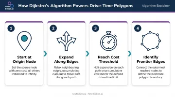
The boundary connecting those frontier points becomes the polygon edge. Modifications to the base Dijkstra implementation handle real-world constraints: one-way streets, turn restrictions, barriers, and side-of-street rules.
Impedance and Network Attributes
The impedance attribute defines what cost the solver accumulates. Switch from a TravelTime impedance (minutes per segment) to a distance impedance (miles or kilometers), and the same traversal produces a drive-distance polygon instead.
Custom network attributes can be layered on top: vehicle weight limits, height restrictions, hazmat routing, urban road class exclusions. Each constraint changes which edges the solver can traverse — and therefore changes the polygon shape.
Polygon Geometry Construction and Configuration
Once traversal completes, the raw output is a set of reached edges. Converting those edges into a usable polygon requires several geometry steps:
- Edge endpoints at the cost threshold are projected outward
- A hull (convex or concave) is computed around the reachable area
- Optional smoothing reduces jagged boundaries from dense road grids
Two configuration parameters directly trade off precision against file size:
- Polygon Trim Distance — controls how closely the polygon follows reached network edges (default: 100 meters per Esri documentation)
- Polygon Simplification Tolerance — reduces vertex count; larger values produce smaller files but less accurate boundaries at high zoom
Production Deployment Limits
For teams building polygon generation services, Esri's Generate Service Areas tool documents these constraints:
- Maximum facilities: 1,000 per request
- Maximum break value: 300 minutes or 300 miles
- Detailed polygon limit: 15 minutes or 15 miles
- Credit cost: 0.5 credits per service area when using ArcGIS Online network data
Hitting the 15-minute detailed polygon ceiling is a common surprise in production — anything beyond that threshold drops to generalized geometry, which affects accuracy for tight service-area calculations.
Business Use Cases for Drive-Time Polygons
Last-Mile Delivery and Delivery Zone Design
Capgemini's research found that last-mile delivery accounts for 41% of total supply-chain costs — making zone design one of the highest-leverage decisions a logistics operator makes.
Drive-time polygons change how zones are built:
- Compute 15-, 30-, and 45-minute polygons around each depot to create tiered delivery zones
- Assign order volumes per zone based on realistic driver capacity, not assumed radius coverage
- Set delivery fee structures that reflect actual drive time rather than straight-line distance
- Identify where circular zones over-assign orders to drivers facing congested corridors
The practical gap between a circular zone and a drive-time polygon widens considerably in cities with rivers, rail infrastructure, or limited highway on-ramps — exactly the environments where misallocation costs show up most clearly.
Field Service Territory Planning
Field service businesses — pest control, HVAC, utilities — define technician territories based on how far a tech can realistically travel from their home base in a working shift. A drive-time polygon from each technician's starting location creates a service zone that reflects actual road access. When zones from different technicians are overlaid, coverage gaps become visible immediately.
Managers can then adjust territories based on road network reality, not geometric assumptions. Hawx Pest Control, a NextBillion.ai customer, uses the platform's routing APIs for technician scheduling and job allocation — reducing developer hours spent on manual scheduling while cutting time dispatchers spend resolving territory conflicts.
Retail Site Selection and Market Coverage Analysis
Retailers and franchise operators evaluate candidate locations by overlaying drive-time polygons with demographic data. A 20-minute polygon from a proposed site that contains fewer than a target household count fails the accessibility threshold — no amount of marketing changes the road network.
Multiple polygons from competing store locations reveal cannibalization risk: where two 20-minute polygons overlap, customers are equidistant from both stores. Esri's Business Analyst tools explicitly support this workflow, allowing demographic and spending data to be appended directly to generated trade-area polygons.
Emergency Response and Healthcare Access
NFPA 1710 specifies first-engine arrival at 240 seconds for career fire departments. A 4-minute drive-time polygon from a fire station shows exactly which neighborhoods meet that standard — and which fall outside it.
Healthcare planners use the same approach. Medicare Advantage network adequacy standards (42 CFR 422.116) define maximum time and distance thresholds by county type and provider specialty. Overlaying patient population data with facility-based drive-time polygons identifies where access gaps exist before they become compliance or service failures.
How to Generate Drive-Time Polygons
Desktop GIS Platforms
Two common desktop approaches:
- ArcGIS Pro + Network Analyst — Generate Service Areas tool using a local or online network dataset; requires a Network Analyst license; consumes 0.5 ArcGIS Online credits per service area when using cloud network data. Best for one-off analysis projects.
- QGIS plugins — ORS Tools (calls the openrouteservice API using OpenStreetMap data; requires an API key) and TravelTime (calls the TravelTime API; outputs temporary vector polygon layers). Both return isochrone geometries usable in QGIS workflows.
Desktop tools work well for periodic analysis. For programmatic or high-volume generation, an API-based approach is the only viable path.
API-Based Generation for Production Systems
When polygons need to be generated dynamically — on order creation, territory refresh, demand change, or driver assignment — an API is the only viable architecture. Each request includes:
- Origin coordinates
- Cost type (time or distance)
- Cost value (e.g., 30 minutes)
- Vehicle type (car, van, truck)
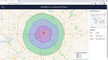
The API returns a GeoJSON polygon that can be rendered on a map, stored in a database, or piped into downstream spatial queries.
NextBillion.ai's Isochrone API is built for logistics and field service teams that need drive-time polygons at volume. Its technical capabilities cover routing fidelity and data quality:
- Supports time-based and distance-based polygons across all vehicle profiles
- Truck-specific routing constraints — weight limits, height restrictions, hazmat routing, road class exclusions — so polygon shapes reflect what a specific vehicle can actually reach
- Road network sourced from OpenStreetMap and TomTom, updated quarterly (faster updates available on request)
- Live traffic integrated into reachability calculations
- Custom road attributes via the Road Editor App: speed overrides, turn restrictions, no-entry zones, and time-of-day rules that feed directly into isochrone calculations
On the operational and commercial side:
- GeoJSON output, compatible with standard mapping and spatial database workflows
- Available via cloud (North America, Europe, Asia) or on-premise deployment within a customer's own Kubernetes environment or private data center
- Per-vehicle or per-order pricing rather than per-API-call billing, removing the cost unpredictability common with general-purpose mapping providers
- Free trial API key available for 1–2 weeks with solutions engineering support
The Isochrone API connects directly to NextBillion.ai's Route Optimization, Distance Matrix, and Clustering APIs. Territories defined by isochrones feed straight into route planning and task assignment, with no data handoff between separate platforms.
What Affects Drive-Time Polygon Accuracy?
Road Network Data Quality
The network graph is the foundation. Missing road segments, outdated speed limits, or incorrect turn restrictions all produce polygons that misrepresent reachable area. The gap between Euclidean and road-network measures has been documented at approximately 146 miles in sparse or barrier-heavy networks — a margin that can invalidate an entire territory design.
Providers differ in data freshness, OSM contribution monitoring, and handling of local conditions like private roads, seasonal closures, and weight-restricted access.
Traffic Modeling
Three traffic model types produce materially different polygon shapes:
- Static model — uses posted speed limits or fixed averages; produces the same polygon at 8 a.m. and 8 p.m.
- Historical peak/off-peak model — uses averaged speed observations by day and time; reliable for recurring planning scenarios
- Live/real-time model — incorporates current conditions from road sensors and GPS data; appropriate for live dispatch but can be noisy for planning
For territory design and zone planning, a stable historical model often outperforms real-time data — live feeds introduce noise that distorts repeatable planning. Dispatch operations are the exception, where current conditions are exactly what matters.
Vehicle Type and Routing Constraints
An auto polygon and a truck polygon from the same origin look different — sometimes dramatically so. Heavy vehicles cannot use roads with weight limits, low clearances, or urban delivery restrictions. A standard auto profile applied to a truck fleet generates polygons that include roads the vehicles physically cannot traverse.
For fleet operators, the wrong vehicle profile doesn't just affect one route — it introduces systematic errors into every zone and territory decision built on those polygons, compounding across hundreds of stops.
Frequently Asked Questions
What is the difference between a drive-time polygon and a simple radius circle?
A radius circle assumes equal travel speed in every direction regardless of roads, terrain, or barriers. A drive-time polygon follows the actual road network, producing an irregular shape that reflects where a driver can genuinely reach within the given time. The practical difference can be substantial in areas with rivers, rail lines, or limited highway access.
How are drive-time polygons used in logistics and delivery operations?
Logistics operators compute tiered polygons (such as 15, 30, and 45 minutes) around depot locations to define delivery zones, assign order volumes to drivers based on realistic capacity, and set accurate delivery fee structures. This prevents the zone misalignment that occurs when circular zones ignore road density differences across directions.
What is the difference between drive-time and drive-distance polygons?
Both use network traversal against the same road graph — the difference is the cost attribute. Drive-time polygons measure minutes; drive-distance polygons measure miles or kilometers. Time-based polygons suit scheduling-constrained operations; distance polygons are better for fuel cost or vehicle range scenarios.
Can drive-time polygons account for real-time traffic conditions?
It depends on the platform. Some use static speed models, others use historical peak/off-peak profiles, and some incorporate live traffic data. For territory planning, a historical model typically provides more consistent results, since zones tied to rush-hour traffic will shift throughout the day. For live dispatch decisions, such as reassigning a same-day delivery when a driver falls behind, real-time traffic integration produces more accurate reachability.
What data inputs are needed to generate a drive-time polygon?
Minimum inputs: origin coordinates, cost type (time or distance), and cost value (such as 30 minutes). Optional inputs include vehicle type and travel mode, which matter because a truck restricted from residential streets or with lower speed limits reaches a smaller area than a car in the same time. The underlying road network dataset is provided by the platform — users don't supply it.
How many drive-time polygons can be generated simultaneously in a production system?
Desktop GIS tools are limited to small batches and manual workflows. API-based services support concurrent requests across multiple origins and are necessary for any production system generating polygons at fleet scale — especially platforms built for logistics, which add truck-specific routing constraints and predictable pricing that general GIS tools don't offer.
How do you calculate drive time?
Drive time is calculated by running a routing engine against a road network graph, where each road segment carries a cost based on speed limit, road class, and sometimes historical or live traffic. The engine finds the fastest path from an origin to every reachable point, and drive-time polygons trace the outer boundary of points reachable within a set number of minutes, following actual roads rather than straight-line distance.
How far can I drive in 30 minutes?
There's no fixed distance — it depends entirely on road network, speed limits, and traffic in the specific area. In a dense urban core, 30 minutes might cover a few miles; on a rural highway network, it could cover 30 miles or more. This is exactly why drive-time polygons are used instead of a fixed-radius circle: they map the real reachable area rather than assuming a constant speed.