Introduction
Every delivery operation, field service team, and logistics planner eventually faces the same question: who can we actually reach — and in how long? The instinctive answer is to draw a circle on a map. But circles lie. They ignore highways, rivers, traffic, and the reality that five miles through a city grid is not the same as five miles on an interstate.
Isochronous catchment areas fix that problem. Instead of measuring straight-line distance, they map every point reachable from an origin within a given travel time — following actual roads, respecting actual speeds.
Research from a 2022 PMC study found that Euclidean (straight-line) buffers can bias exposure estimates by -80% to -20% compared to road-network methods — a range large enough to make delivery zone definitions, territory assignments, and facility siting decisions meaningfully wrong.
This guide walks through the full calculation process: definitions, required inputs, the five-step method, accuracy parameters, and the common mistakes that produce misleading results.
Key Takeaways
- An isochronous catchment area is a road-network polygon showing all locations reachable within a set travel time — not a circle.
- You need: precise origin coordinates, a routing engine or isochrone API, and a population/demand dataset.
- Five steps take you from a raw origin point to an enriched, analyzable catchment polygon.
- Accuracy hinges on travel mode, time thresholds, road data quality, and live traffic conditions.
- Common mistakes: using radius buffers, applying a single threshold, and skipping population enrichment.
What Is an Isochronous Catchment Area?
The term comes from the Greek iso (equal) + chronos (time). An isochronous catchment area is a geographic polygon enclosing all points reachable from a defined origin within an equal travel time.
Three methods are commonly confused:
| Method | What It Measures | Accounts for Roads? |
|---|---|---|
| Radius buffer | Straight-line distance | No |
| Isodistance | Road-network distance | Yes, but not speed |
| Isochrone | Travel time via road network | Yes (mode, speed, and traffic) |
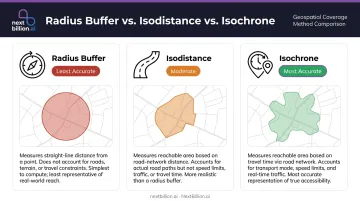
The practical difference is significant. A 15-minute isochrone in a dense urban grid extends much shorter distances than a 15-minute isochrone near a highway interchange — because the road network, not the ruler, determines what's reachable.
Why This Matters for Operations
That road-network reality has direct operational consequences. For delivery and field service teams, travel time drives cost — not distance. A technician is paid by the hour, not the mile. Defining territories and service zones by time-based catchments produces more balanced workloads and more reliable SLA commitments than any distance-based alternative.
Common applications include:
- Defining delivery zones for same-day and scheduled fulfillment
- Designing field service territories for technicians, pest control teams, and repair crews
- Siting facilities for retail, healthcare, or depot location decisions
- Planning franchise territories where non-overlapping coverage is contractually required
What You Need Before Calculating Isochronous Catchment Areas
The quality of your catchment output depends entirely on what goes in. Most inaccurate catchments trace back to a rushed setup — wrong coordinates, undefined objectives, or the wrong routing tool for the job.
Origin Point and Objective Clarity
You need precise geographic coordinates — latitude and longitude — for each origin point: a store, warehouse, depot, or technician home base. Coordinate accuracy matters. A misplaced pin shifts every boundary that follows.
Before running any calculation, define your business objective:
- Are you setting delivery zones for same-day fulfillment?
- Designing technician territories for a field service operation?
- Evaluating candidate locations for a new facility?
- Modeling healthcare access for underserved populations?
The objective determines which travel mode and time thresholds are appropriate. A healthcare access analysis uses different parameters than a last-mile logistics zone.
Routing Engine or Isochrone API
You need access to a routing engine that generates isochrone polygons from coordinates. Options include:
- OpenRouteService (ORS) — supports time and distance isochrones, returns GeoJSON; public API limited to 5 locations and 1-hour driving ranges
- Valhalla — supports auto, bicycle, pedestrian, and multimodal costing; up to 4 contours per request by default
- OSRM — high-performance routing engine, but its official API does not expose an isochrone endpoint
- Production APIs (NextBillion.ai, TomTom, HERE): built for high-volume, programmatic isochrone generation with traffic-aware routing and enterprise SLAs
Open-source tools suit exploratory analysis or low-volume use. Operations that need to calculate catchments programmatically across dozens or hundreds of origin points require a production-grade API.
Population or Demand Data
A raw isochrone polygon defines geography. To make it actionable, you need a dataset to intersect with it:
- Census block-group population counts (ACS 5-year estimates, available down to groups of 600–3,000 people)
- Household income or demographic data
- Existing customer records
- Demand density or points-of-interest data
With these three inputs in place — a verified origin point, a routing engine matched to your use case, and a relevant demand dataset — you're ready to run your first isochrone calculation.
How to Calculate Isochronous Catchment Areas: Step-by-Step
Calculating a catchment area is iterative — you define inputs, generate the polygon, enrich it with data, and refine. Each step builds on the previous one.
Step 1: Define Your Origin Point and Business Objective
Input your coordinates (latitude, longitude) for each origin location. If you're calculating catchments for multiple sites — depots, stores, technician zones — each gets its own origin point.
Document your objective before running anything:
- Same-day delivery radius? → You need a driving isochrone with traffic conditions for your delivery window.
- Technician territory assignment? → You need a driving isochrone calibrated to your dispatch hours.
- New branch coverage analysis? → You may need multiple nested thresholds to compare site options.
Skipping this step is how teams end up regenerating polygons three times because the first two answered the wrong question.
Step 2: Select Travel Mode and Set Time Thresholds
Travel mode must match how people or vehicles actually move:
- Driving for delivery fleets, field service, and most logistics operations
- Walking or cycling for urban retail access or last-mile pedestrian analysis
- Public transit for healthcare access or workforce availability studies
Mixing modes or selecting the wrong one produces a polygon that doesn't represent operational reality.
Once you've confirmed the right mode, set time thresholds as nested intervals rather than a single boundary. For example:
- 10 / 20 / 30 minutes for delivery zone prioritization
- 15 / 30 / 45 minutes for field service territory design
Nested isochrones show how coverage degrades with distance — a location 5 minutes out and a location 29 minutes out are not equivalent, even if both fall inside a single 30-minute boundary.
Step 3: Generate the Isochrone Polygon
The routing engine expands outward from the origin along the road network, marking every point reachable at each time threshold, then connects those boundary points into a polygon. This process relies on shortest-path graph algorithms (Dijkstra-based expansion across a weighted road network), with faster preprocessing methods like Contraction Hierarchies used in production systems.
Output is typically a GeoJSON polygon you can load into GIS tools, BI platforms, or downstream planning systems.
For logistics, delivery, or field service teams calculating isochrones across many origin points, a production-grade API handles this at scale. NextBillion.ai's Isochrone API generates road-network-accurate polygons with support for real-time and historical traffic, vehicle-specific routing constraints (truck dimensions, weight limits, hazmat restrictions), and custom road attributes. That combination makes it practical to embed catchment logic directly into dispatch systems or territory management workflows.
Step 4: Overlay and Intersect with Population or Demand Data
Perform a spatial join between the isochrone polygon and your data layer. This is what converts a shape into a business insight.
Practical approach:
- Load your isochrone polygon and your census/demand dataset into a GIS tool or spatial database
- For efficiency, use centroids of the underlying census block groups rather than full polygon-on-polygon intersection
- Sum population values of all units whose centroids fall within the isochrone
- Aggregate to get catchment population, household count, or demand estimate
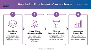
The Census Bureau's TIGER/Line shapefiles provide geographic boundaries; the ACS 5-year data provides the demographic values. These need to be joined — the shapefiles alone contain no population data.
Step 5: Analyze, Validate, and Refine
Examine the output against local knowledge. Does the boundary make sense?
Flag these anomalies:
- A catchment that crosses a river with no bridge
- Coverage extending through a restricted or impassable zone
- An implausibly large or small area relative to expectations
These typically indicate a routing engine problem or an input error — not a business reality.
If the result doesn't match known customer behavior or operational constraints, adjust your time thresholds or travel mode and regenerate. Document the final parameters so catchments can be reproduced consistently when territories are reviewed or new locations are added.
Key Parameters That Affect Results
Two teams using the same origin point can get meaningfully different catchments depending on how these variables are configured.
Travel Mode
The gap between modes is larger than most people expect. A walking isochrone uses a default speed around 5 km/h; a driving isochrone follows road network speeds. Choose the mode that reflects how your operation actually works — not the mode that produces the most favorable polygon.
For trucking operations, vehicle-specific routing becomes critical: a heavy goods vehicle restricted to certain roads has a smaller reachable area in the same time window than a car or a delivery motorcycle.
Time Threshold Granularity
A single boundary (e.g., "30 minutes") hides how coverage tapers. Nested intervals give planners the ability to:
- Identify a high-priority inner zone (e.g., 10 min) for premium delivery commitments
- Assign standard service to a mid-zone (e.g., 20 min)
- Flag outer zones (e.g., 30 min) for surcharge or partner fulfillment
Three to four intervals typically provide useful granularity without visual complexity. Most isochrone APIs, including ORS and Valhalla, support multiple thresholds per request.
Road Network Data Quality
The polygon is only as accurate as the underlying road data. Outdated maps that miss new roads, fail to reflect access restrictions, or omit turn restrictions generate polygons that look correct but don't match reality.
A 2017 study estimated global OSM street-network completeness at approximately 83%, with significant variation by region. For enterprise operations in complex urban or industrial corridors, road data recency is not a minor consideration: it directly determines whether your service zones reflect what's actually drivable.
That data quality gap is why NextBillion.ai uses OpenStreetMap and TomTom as dual data sources, with quarterly map updates and the ability to swap data sources by territory for best coverage.
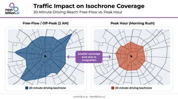
Time-of-Day and Traffic Conditions
A 20-minute driving isochrone at 2 AM covers substantially more area than the same isochrone during morning peak hours. FHWA defines congested hours as periods when travel speeds fall below 90% of free-flow speed, and those periods can significantly compress what's operationally reachable.
Static, free-flow isochrones are appropriate only when timing is irrelevant. For delivery windows, technician dispatch, and any time-sensitive operation, traffic-aware routing is necessary. Verify whether your API supports departure-time-based routing before using it for operational planning.
Common Mistakes When Calculating Isochronous Catchment Areas
Using a radius buffer instead of an isochrone — A circular buffer ignores roads, rivers, and terrain. The PMC research cited earlier documented how this can bias estimates by up to 80% — one example found 14 destinations inside a Euclidean buffer where only 5 were actually reachable by road.
Applying a single time threshold — A single boundary treats a location 3 minutes away the same as one 29 minutes away. For delivery zone prioritization or territory design, this leads to over-promising windows and territories that are too large in practice.
Skipping population enrichment — A polygon with no data layer is a shape, not an insight. The spatial join step is what connects geography to market size, operational workload, or customer density.
Treating catchments as static — Roads open, close, and shift in traffic patterns seasonally. Catchments calculated once and never revisited produce increasingly unreliable territory assignments over time.
Alternatives to Isochronous Catchment Area Calculation
Isochrones are the most operationally accurate method for most logistics and field service use cases — but other approaches exist and are sometimes appropriate.
| Method | Best For | Key Limitation |
|---|---|---|
| Radius buffer | Rapid first-pass estimates; areas where road network closely tracks straight-line distance | Ignores barriers and road structure; unsuitable for operational zone definition |
| Isodistance | Mileage-constrained zones (fuel cost management, per-mile pricing) | Doesn't account for speed differences across road types |
| Mobility/behavior-based | Trade area validation using observed visit data | Requires expensive mobility datasets; reflects past behavior, not potential reach |
Among these options, isochrones remain the right starting point for greenfield site selection or new territory design. Mobility-based catchments can validate results after the fact — useful for confirming that a proposed territory matches where customers actually come from.
Frequently Asked Questions
How do you calculate a catchment area?
Define an origin point, select a travel mode and time threshold, generate an isochrone polygon using a routing engine or API, and intersect it with population or demand data. The right parameters vary by objective: delivery zone definition, territory design, and facility siting each require a slightly different setup.
What is the difference between an isochrone and a buffer catchment area?
A buffer is a circle drawn at a fixed straight-line distance, ignoring roads, barriers, and terrain. An isochrone traces all points reachable within a given travel time along the actual road network. For any operational planning purpose, isochrones are far more accurate.
What data do you need to calculate an isochronous catchment area?
Three inputs: precise origin coordinates, access to a routing engine or isochrone API that generates road-network-aware polygons, and a population or demand dataset (such as Census ACS data or customer records) to enrich the polygon with business-relevant metrics.
Can isochronous catchment areas account for traffic conditions?
It depends on the routing engine. Basic open-source tools calculate under free-flow assumptions. Advanced commercial APIs support departure-time-based routing with historical and real-time traffic data, producing more accurate catchments for time-sensitive windows like morning deliveries or peak-hour dispatch.
How do you calculate catchment area population from an isochrone?
Intersect the isochrone polygon with a census dataset at the block group level. Use centroids of the census units and sum the population values of all units whose centroids fall within the polygon to get an estimated catchment population figure.
How many time thresholds should an isochrone catchment area use?
Three to four nested thresholds (for example, 10, 20, and 30 minutes) works well for most logistics and service planning. Nested intervals reveal how accessibility tapers off from the origin and let planners prioritize high-density zones — something a single boundary can't show.